Comparing different visualizations for the Worldbank population dataset
Author
Marco Dalla Vecchia
Published
December 6, 2024
In [27]:
from matplotlib import pyplot as pltimport seaborn as snsimport numpy as npimport pandas as pd# Aestheticssns.set_style('ticks')plt.rcParams["font.family"] ="serif"# use Serif style as default font
In [28]:
# Read list of european countries withopen('../data/europe-countries.txt', 'r') as f: lines = f.readlines()countries_europe = [line.replace('\n','') for line in lines]# Import World Bank population datadf = ( pd.read_csv('../data/API_SP.POP.TOTL_DS2_en_csv_v2_320414/API_SP.POP.TOTL_DS2_en_csv_v2_320414.csv', skiprows=3) .drop(columns=['Indicator Code', 'Indicator Name', '2023', 'Unnamed: 68']) .melt(id_vars=['Country Name','Country Code']) .rename({'Country Name':'country-name', 'Country Code':'country-code', 'variable':'year', 'value': 'population'}, axis=1) .assign(year=lambda df_: pd.to_numeric(df_.year)) .loc[lambda df_: df_['country-name'].isin(countries_europe)] .reset_index(drop=True))df
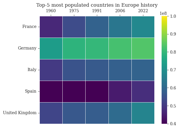
ax = sns.heatmap(df_heatmap, linewidth=.5, vmin=4e7, vmax=10e7, cmap='viridis')ax.set(xlabel="", ylabel="")ax.xaxis.tick_top()ax.set_title("Top-5 most populated countries in Europe history")fig.savefig('../figures/heatmap.pdf', bbox_inches='tight')plt.show()
Figure 3: Heatmap for the visualization of european countries population in different years
Figure 4: Barplot for the visualization of european countries population in different years
In [26]:
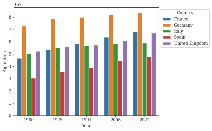
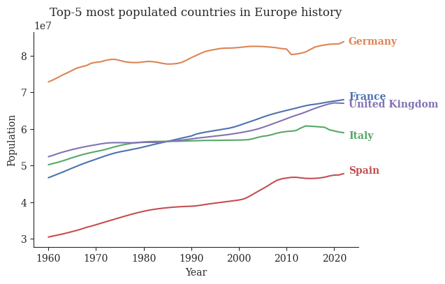
df_lineplot = ( df .loc[lambda df_: (df_['country-name'].isin(top_5_countries)) ] .drop(columns='country-code') .sort_values('country-name'))np.random.seed(100)fig, ax = plt.subplots(1,figsize=(6,4))sns.lineplot(data=df_lineplot, x='year', y='population', hue='country-name', palette='deep', legend=False)for (label, group_df), color inzip(df_lineplot.groupby('country-name'), sns.color_palette('deep', 5)): y_pos = group_df.loc[lambda df_: df_['year'] ==2022]['population'].values[0] + np.random.randint(-1e6, 1e6) x_pos =2023 ax.text(x_pos, y_pos, label, va='center', color=color, fontweight='bold')ax.set_title("Top-5 most populated countries in Europe history")ax.set(xlabel="Year", ylabel='Population')sns.despine()fig.savefig('../figures/lines-time.pdf', bbox_inches='tight')plt.show()
/home/mdallave/miniconda3/envs/data-viz/lib/python3.11/site-packages/seaborn/_oldcore.py:1119: FutureWarning: use_inf_as_na option is deprecated and will be removed in a future version. Convert inf values to NaN before operating instead.
  with pd.option_context('mode.use_inf_as_na', True):
/home/mdallave/miniconda3/envs/data-viz/lib/python3.11/site-packages/seaborn/_oldcore.py:1119: FutureWarning: use_inf_as_na option is deprecated and will be removed in a future version. Convert inf values to NaN before operating instead.
  with pd.option_context('mode.use_inf_as_na', True):
/home/mdallave/miniconda3/envs/data-viz/lib/python3.11/site-packages/seaborn/_oldcore.py:1075: FutureWarning: When grouping with a length-1 list-like, you will need to pass a length-1 tuple to get_group in a future version of pandas. Pass `(name,)` instead of `name` to silence this warning.
  data_subset = grouped_data.get_group(pd_key)
Figure 5: Lineplot for the visualization of european countries population in different years
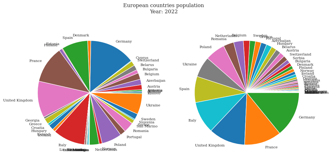
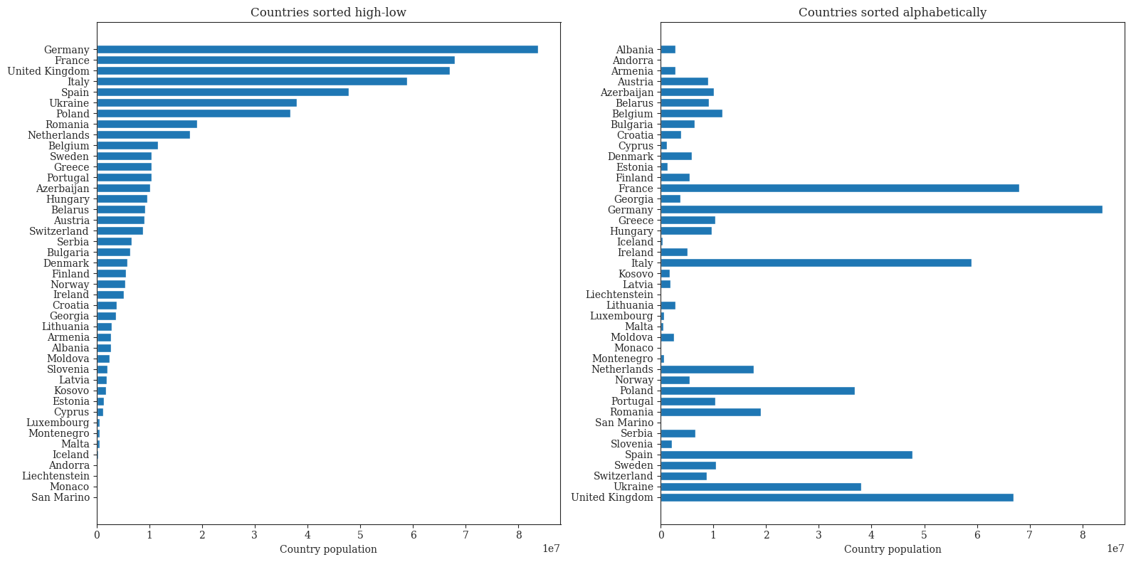
Figure 1: Pie charts for the visualization of european countries populationFigure 2: Bar charts for the visualization of european countries populationFigure 3: Heatmap for the visualization of european countries population in different yearsFigure 4: Barplot for the visualization of european countries population in different yearsFigure 5: Lineplot for the visualization of european countries population in different years